Light curve analysis of exoplanets
Into this section it will be explained step by step how to analyse the light curve of exoplanets.
First, choose a constellation in which you have special interest on analizing its exoplanets.
As soon as you have decided the constellation to work with, open a new tab and search: "NAME OF YOUR CONSTELLATION" + IAU. Then, open the image tool. In there you will find an image of the International Astronomical Union of your constellation in which will be specified its coordinates.
Next, open the Nasa exoplanet archive and go into "Confirmed Planets". There are columns not needed for analizing the light curve, so that click on "Select columns" and only tick:
- Planet Name
- Planet Radius [Jupiter Radius]
- Planet Mass [Jupiter Mass]
- Stellar Radius [Solar Radius]
- Stellar Mass [Solar mass]
- RA [sexagesimal]
- Dec [sexagesimal]
Now, order in increasing or decreasing order the RA column in order to search easily your constellation coordinates. It should look like that:
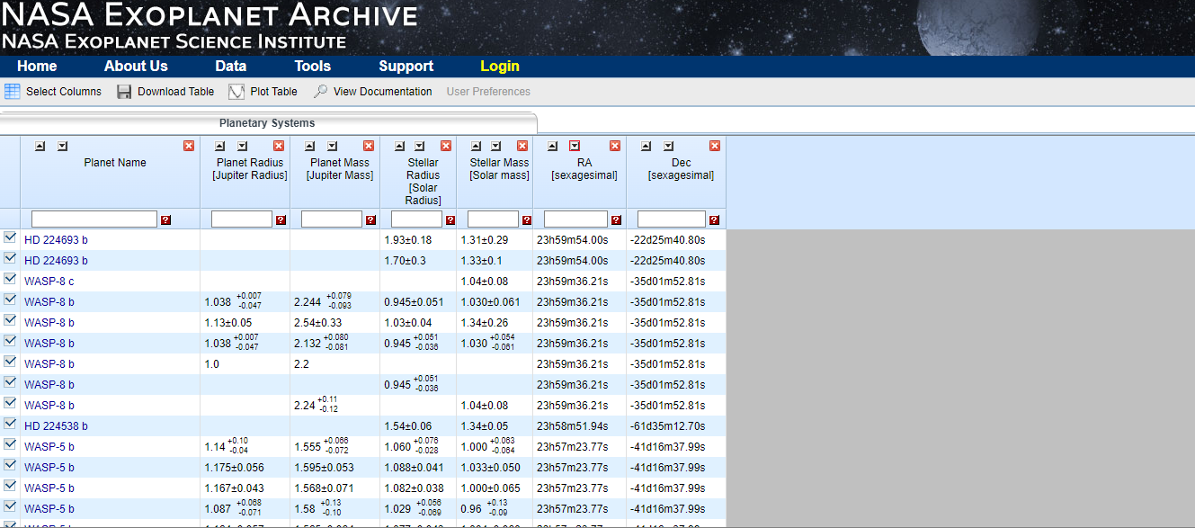
After that, look for exoplanets which match with the coordinates of the constellation and, subsequently, open the Light Kurve Calculation of Nasa and enter the name of the exoplanet.
In the light curve calculator, follow the next steps:
- Provide a name for the calculation (for example, the name of the exoplanet).
- Select "Light Curve File" in the "Data Archive".
- In "Search Parameters" (in the "Target object name") provide once again the name of the exoplanet.
- Select "Simple Aperture Photometry" in "Photometry options".
- At the "Lightcurve Options", select "Normalize" and choose the relative unit "Parts per Million".
- Run the calculation.
- Check the status of the calculation is "Finished". If the status is "Error" revise all the steps or look for another exoplanet.
- Click on "View results"
Now, with the calculation results, calculate the radius of the exoplanet with the following formula:
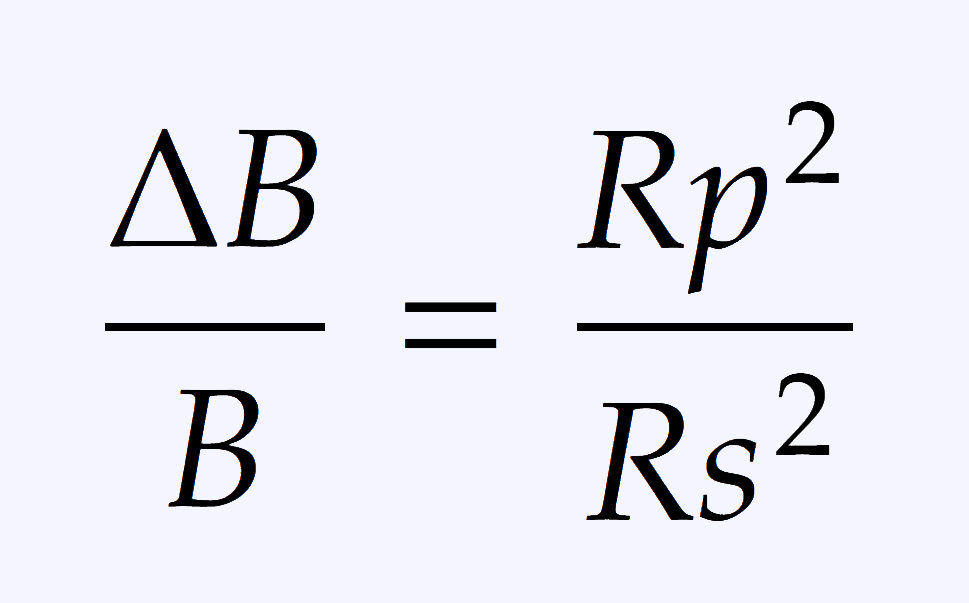
Compare the radius obtained from the previous calculus with scientific articles found at Scholar Google and with data found at Nasa exoplanet archive.
Obtaining mass of exoplanets
To know the planet mass, use the linear regression of exoplanets and the R code found at myComplier (cepheid formula example).
At the RStudio, it is obtained the following graphic.
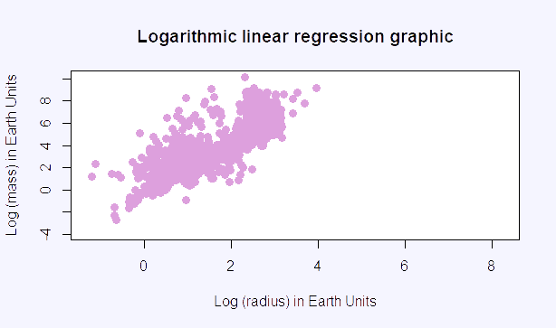
From this graphic, we can create the linear regression, which is a linear approach for modelling the relationship between in this case log (mass) in Earth units and log (radius) in Earth units of the exoplanets. Knowing the radius of the exoplanet, we can obtain its mass.
In the following image there is the calculation of the slope of the linear regression graphic of exoplanets.
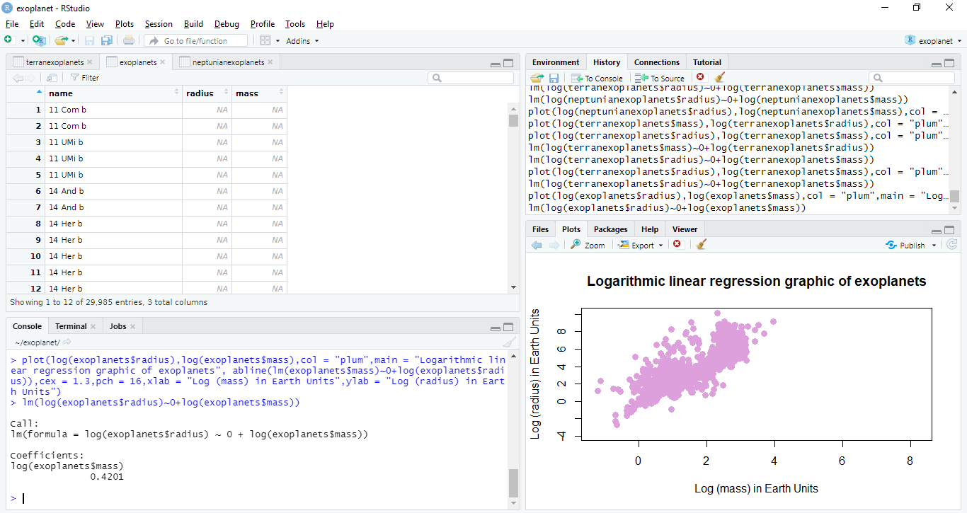
We obtain that the slope of the linear regression graphic of exoplanets is 0.4201.
But actually, the exoplanets should have been divided according their characteristics (Terran worlds, Neptunian worlds, Jovian worlds...) in order to obtain more accurate graphics. Even so, the results obtained with this graphic would approximately correspond to other scientists' results.
The next graphic shows how different are the slopes of linear regression graphic of the different types of worlds.
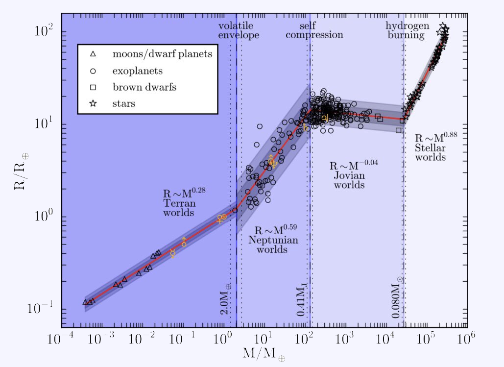
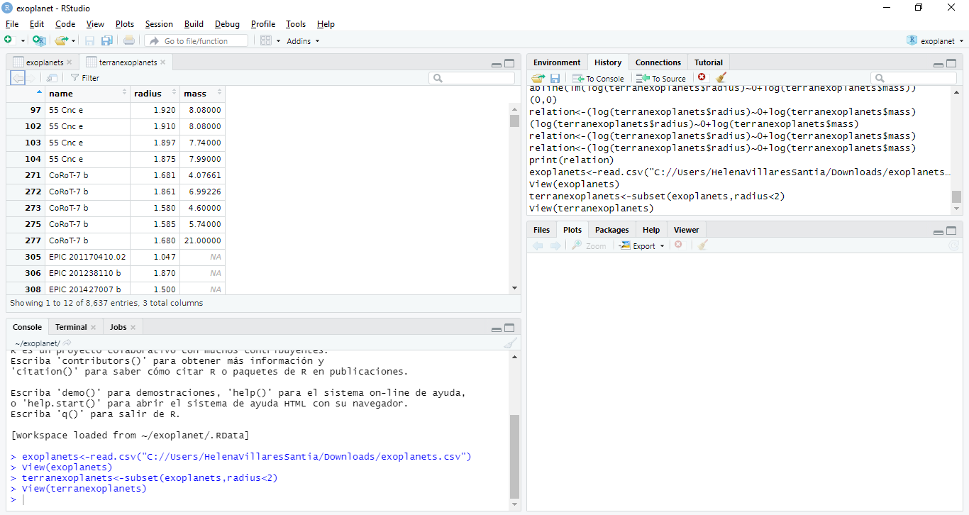
For doing this, we have to include a line in which we are going to make a subset of the planets with the radius smaller than 2 R⊕, because according to the previous graphic, Terran worlds do not have a radius greater than 2 R⊕.
Explaination of the code used in RStudio step by step.
- First, download the data of Planet Radius and Planet Mass, both in Earth Units, at Nasa Exoplanet Archive in CSV fomat and select values only (no errors, limits, etc.).
- Then, read this file in RStudio and create a subset only for Terran worlds as it is made at the following image.
- Establish the following relation between the mass and radius.
- To create the Logarithmic linear regression graphic of Terran worlds with this data, enter the following code.
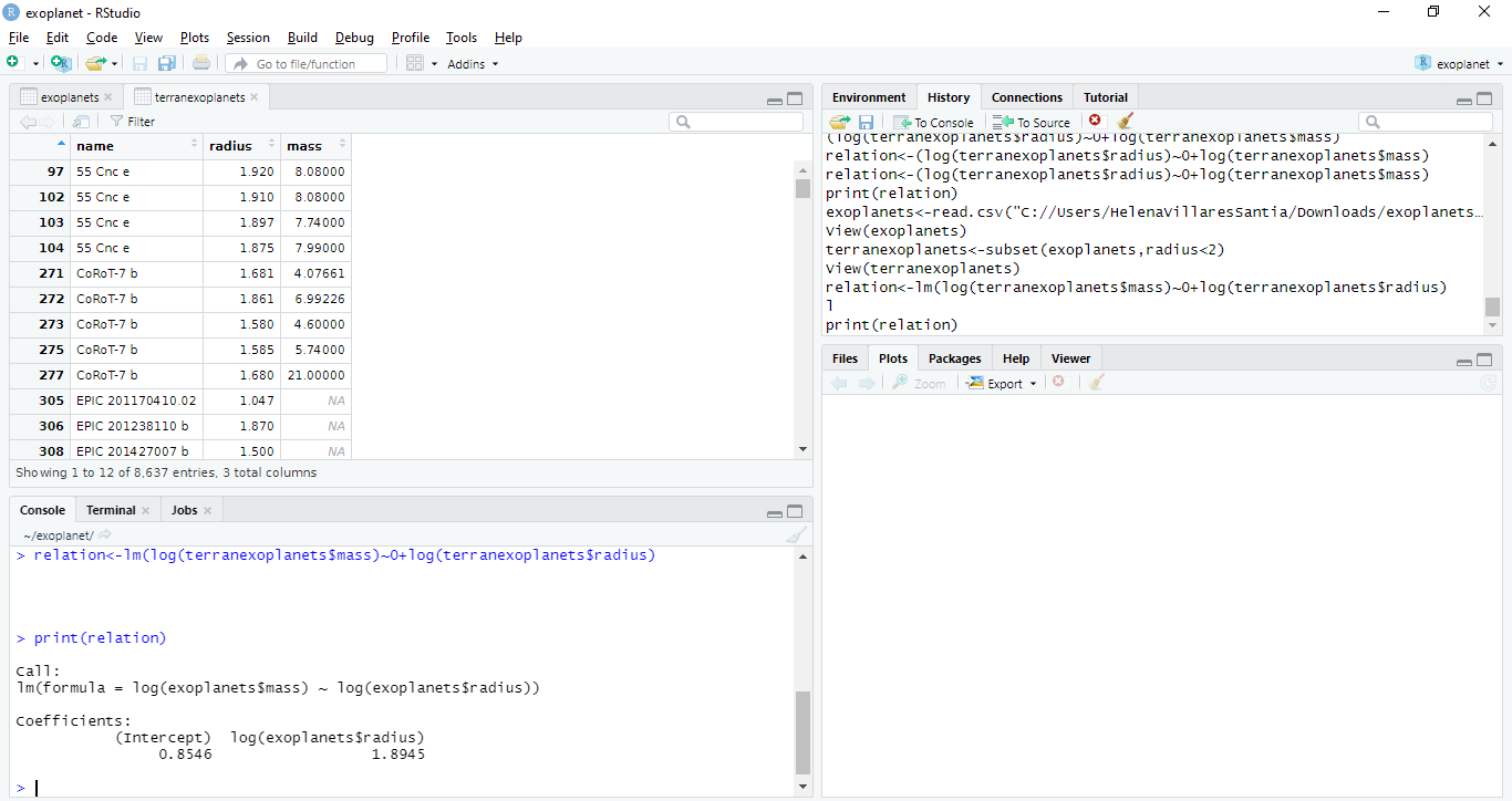
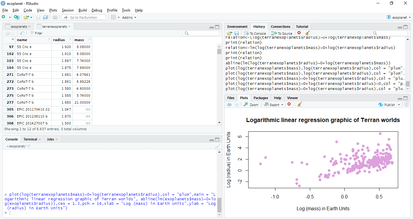
Following this steps, we obtain the following graphic.
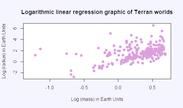
In general, the linear regresion is used to interpole the data of, in this case, the radius of an exoplanet to find its mass. Now that the linear regression graphic of Terran worlds is created, we can obtain the formula for the slope of the line. There are two different ways to obtain it.
The first way is to determine 'a' in consideration of the formula of a line is Y=aX+b, in which 'a' is the slope of the linear regression graphic; 'b', the term that passes through the axis of ordinates, in this case, this line passes through (0,0); Y is the radius in Earth units; and X is the mass in Earth units. Using the following formulae.
In short, as b is zero and Y and X will depend on the exoplanet, we only have to calculate 'a' with the following formula.

The second way is obtaining the slope from RStudio as in the following image.
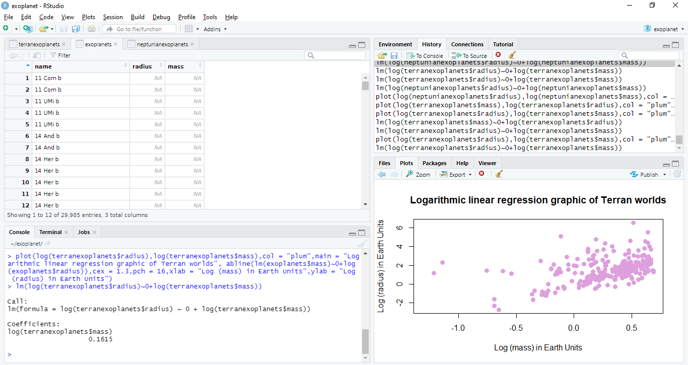
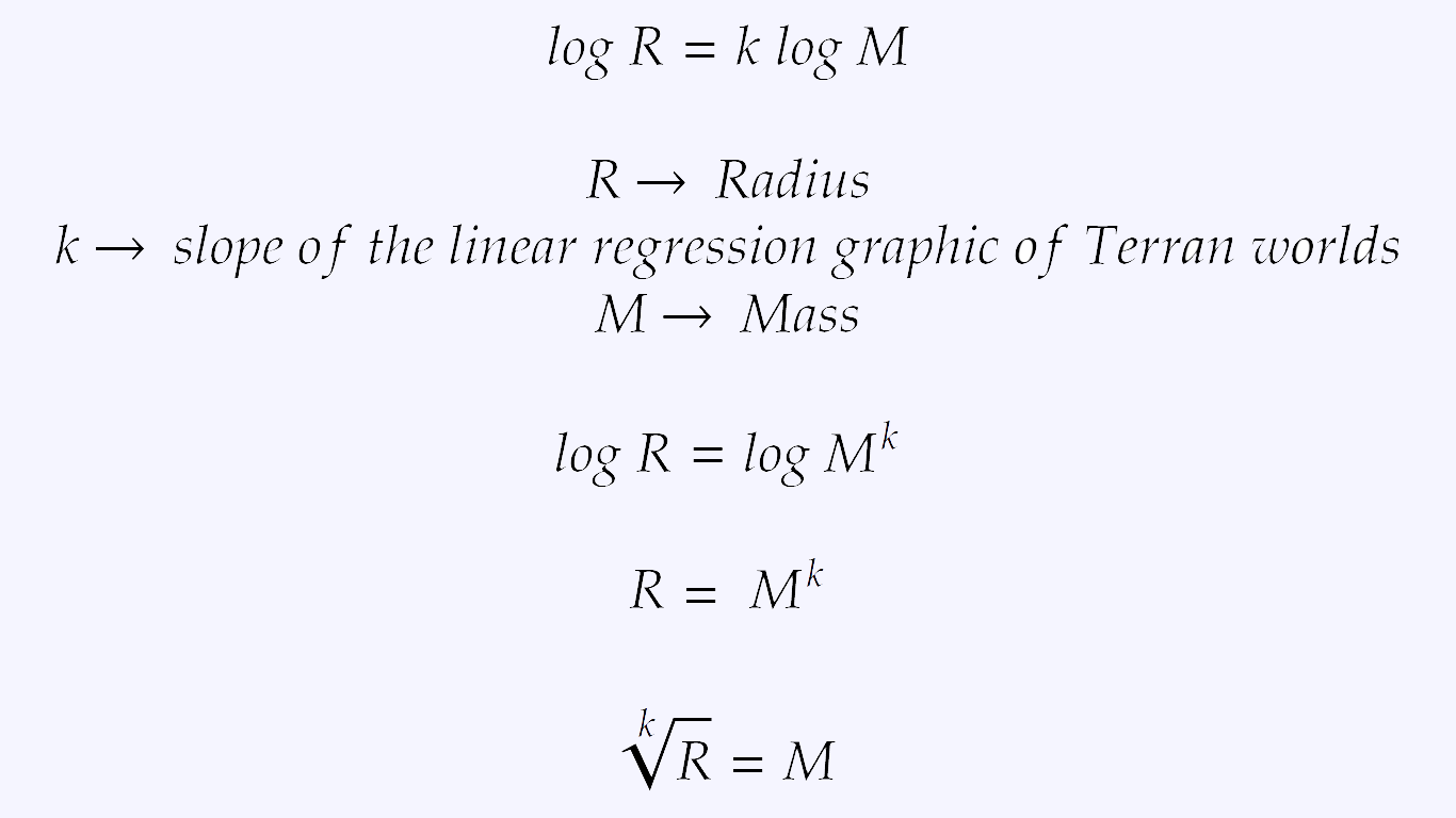
We obtain that the slope of the linear regression graphic of Terran worlds is 0.1615. Now that we have obtained this data, we have to replace it in the following formula.
Calculation of the slope of the linear regression graphic of Neptunian worlds:
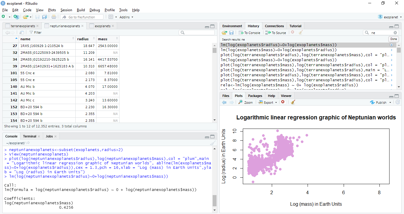
We obtain that the slope of the linear regression graphic of neptunian worlds is 0.4256. Now that we have obtained this data, we have to replace it in the following formula.
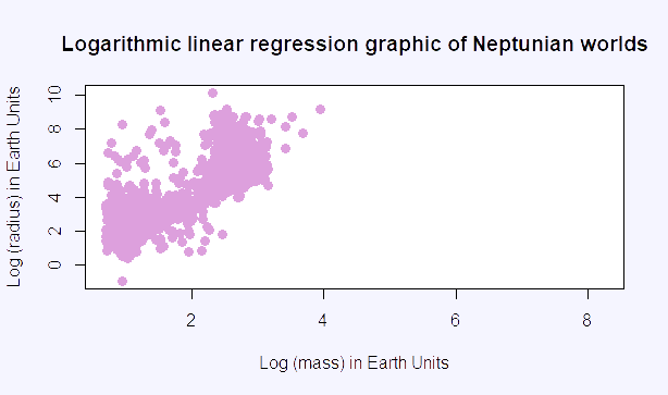
Linear regression graphic of Neptunian worlds
