Analysing air pollution data of Sant Andreu de la Barca

Into this section it will be explained, step by step, the way in which millions of data has been ordered and analysed.

The purposes of the analysis of the air data are:

• Determine wheter Sant Andreu de la Barca, a Municipality in Catalonia, Spain, is in the recommended limits of pollution of Europe and WHO
• To make different graphics with the data obtained in GenCat with RStudio.

1. Obtaining data

The houly data is going to be downloaded for pollution and the half-hourly meteorological data.

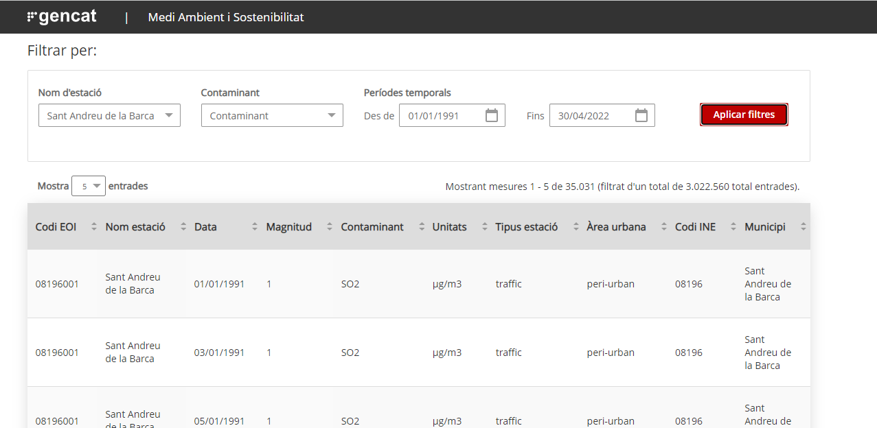
In GenCat it can be found the hourly data of the pollutants measured at the automatic measuring points of the Air Pollution Monitoring and Forecasting Network from 1991 until the day before the current day.

When it comes to the meteorogical data, they can be downloaded at XEMA Meteorological Data. As Sant Andreu does not have any meteorological data, it has been downloaded Castellbisbal ones, a near Municipality.

At the section of filters, variable and station codes must be defined so as not to download wind data of other Municipalities.

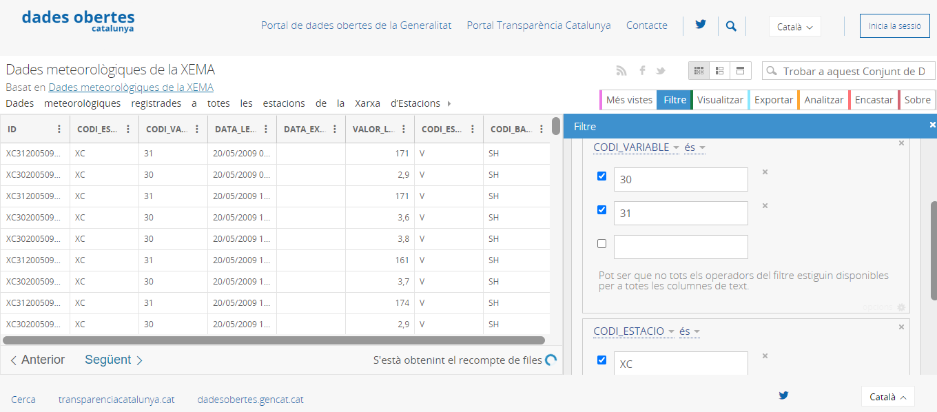
Then, a copy of this set data is downloaded in CSV format.

2. Materials

To order all the data, RStudio must be downloaded.

First it is needed to install some libraries to manipulate and analyse data. The libraries used are the following ones: openair, tidyverse, lares and dplyr.

  > install.packages(c("openair","tidyverse", "lares"))  

3. Methods

# First you need to install some libraries to manipulate and analyse dara
> install.packages(c("openair","tidyverse", "lares"))
# Remember to edit the next line in order to use your city data
# Do not use my hourly data from Martorell
> city<-read.csv('wherever/city.csv')
# You need to call tidyverse library in order to use pivot_longer
> library (tidyverse)
# pivot_longer allows you to convert hour columns to hour rows
> city1<-pivot_longer(city,cols=c(h01,h02,h03,h04,h05,h06,h07,h08,h09,h10,h11,h12,h13,h14, h15,h16,h17,h18,h19,h20,h21,h22,h23,h24), names_to="hour", values_to = "value")
# Delete unnecessary columns
> city2<-city1[-c(1,2,4,6:16)]
# You need dplyr library from tidyverse to use pipe symbol %>% and combine two columns in one
> library(dplyr)
> city2 <- city2 %>% mutate(date=paste0(data, " ", hour))
# check the names of your columns
> colnames (city2)
# delete some unnecessary columns
> city2<-city2[-c(1,3)]
# reorder the columns
> city2<-city2[,c(3,1,2)]
# rename the columns names
> colnames (city2)<-c("date","pollutant","value")
# check changes of column names are correct
 class (city2)
# convert city2 to a dataframe
> city2 <- as_data_frame(city2)
# call lares library to find and replace some values including NA
> library (lares)
> city2<-replaceall(city2, c("T00:00:00.000 h01", "T00:00:00.000 h02","T00:00:00.000 h03","T00:00:00.000 h04","T00:00:00.000 h05","T00:00:00.000 h06","T00:00:00.000 h07","T00:00:00.000 h08","T00:00:00.000 h09","T00:00:00.000 h10","T00:00:00.000 h11","T00:00:00.000 h12","T00:00:00.000 h13","T00:00:00.000 h14","T00:00:00.000 h15","T00:00:00.000 h16","T00:00:00.000 h17","T00:00:00.000 h18","T00:00:00.000 h19","T00:00:00.000 h20","T00:00:00.000 h21","T00:00:00.000 h22","T00:00:00.000 h23","T00:00:00.000 h24"), c(" 01:00:00", " 02:00:00", " 03:00:00", " 04:00:00"," 05:00:00", " 06:00:00"," 07:00:00", " 08:00:00"," 09:00:00", " 10:00:00"," 11:00:00", " 12:00:00"," 13:00:00", " 14:00:00"," 15:00:00", " 16:00:00"," 17:00:00", " 18:00:00"," 19:00:00", " 20:00:00"," 21:00:00", " 22:00:00"," 23:00:00", " 00:00:00"))
# Call openair library to use built-in functions
> library(openair)
# Convert date column from characters to dates
> city2$date<-as.POSIXct(city2$date,"%Y-%m-%d %H:%M:%S", tz="Europe/Madrid")
# Check date column now is a date or POSIXct
> class(city2$date)
# Convert pollutant column from numeric to factor
> city2$pollutant<-as.factor(city2$pollutant)
# Check previous conversion is ok
> class(city2$pollutant)
# To know the different levels of the factor pollutant in order to draw figures
> levels(city2$pollutant)
# Create a figure with hour, day, week, month variations of pollutants
> timeVariation(city2, pollutant=c("O3","NO2","H2S","NO","HCNM","CO","SO2","HCT", "NOX","PM10"), main="Air pollution in Martorell (1991-2022)")
# Create another view of the previous data centered in one pollutant
> trendLevel(city2, pollutant = "H2S", main="Hydrogen sulfide evolution in Martorell")
# Calculate daily means from hourly data of poly
> daily<-timeAverage(city2NO2,avg.time = "day")
> View(daily)
# Create a calendar plot showing values of pollutants with colours
> calendarPlot(daily, pollutant="NO2", year="2021")
# Select only one pollutant of my database
> city2NO2 <- subset(city2, pollutant=="NO2")
# Calculate yearly means from previous data
> yearly<-timeAverage(city2NO2,avg.time = "year")
> View(yearly)
> wind<-read.csv("https://raw.githubusercontent.com/drfperez/openair/main/wind.csv")
# Remember to put your data instead of Martorell default data
> View(wind)
# View your data
> wind1<-wind[-c(1,2,5,7,8)]
# Delete some unnecessary columns
> wind2<-pivot_wider(wind1,names_from = CODI_VARIABLE, values_from = VALOR_LECTURA)
# Convert rows containing wind data in columns
> names(wind2)[names(wind2) == "31"] <- "wd"
# Rename column name to wd (wind direction)
> names(wind2)[names(wind2) == "30"] <- "ws"
# Rename column name to ws (wind speed)
> names(wind2)[names(wind2) == "DATA_LECTURA"] <- "date"
# Rename column name to date (compulsory name for openair library)
> write.csv(wind2,"C:\\Users\\YOURCOMPUTERNAME\\Documents\\wind3.csv")
# Have a copy of ordered original csv data in your local computer.
> wind3<-timeAverage(wind2, time.avg="hour") 
# Combine two databases in one database.
> cityall<-merge(city2, wind3, by ="date")
# Remember to edit the path to be used in your computer
> write.csv(cityall,"C:\\Users\\YOURCOMPUTERNAME\\Documents\\cityall.csv")
> View (cityall)
> pollutionRose(cityall, pollutant="O3")

  

4. Results

From the different codes, there are obtained the following graphics.

timeVariation

  timeVariation(filter(mydata, ws > 3,  wd > 100, wd < 270),pollutant = "pm10", ylab = "pm10 (ug/m3)")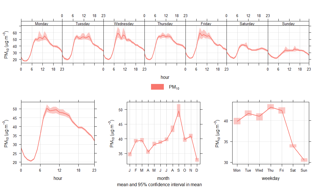  

timeVariation

  timeVariation(mydata, pollutant = "pm10", statistic = median,col = firebrick)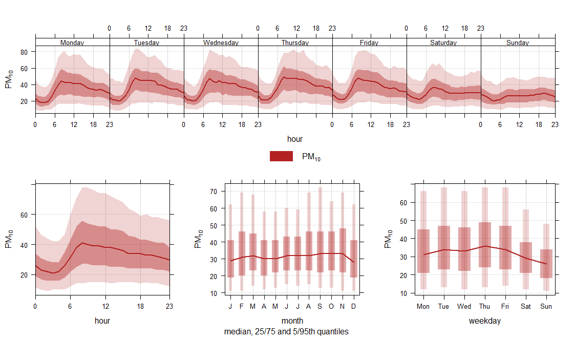  

timeVariation

  mydata <- mutate(mydata,feature = ifelse(ws > 4 & wd > 0 & wd <= 180, "easterly", "other"))
  timeVariation(mydata, pollutant ="so2", group = "feature",  ylab = "so2 (ppb)",difference = TRUE)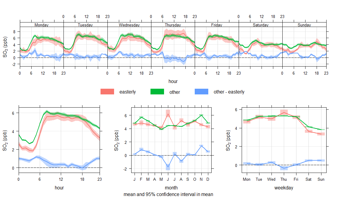  

timeVariation

  source('C:/Users/HelenaVillaresSantia/Desktop/BACHILLERATO/1º BACHILLERATO/3er TRIMESTRE/CMC/city/dataanalysis.R')
  timeVariation(mydata, pollutant = c("nox", "no2", "o3", "pm10", "so2"), main="Air pollution (µg/ m3) in Sant Andreu de la Barca (1991-2022)", normalise = TRUE)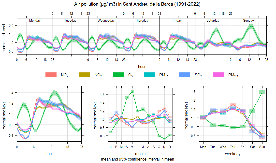  

trendLevel

shows the evolution of the pollutant PM10 over a period of time in the city of Sant Andreu de la Barca. We can see the absence of data in different months over the years, which makes it difficult to make a correct analysis of the real situation in the city.

  trendLevel(mydata, pollutant = "o3", main="Ozone evolution in Sant Andreu de la Barca")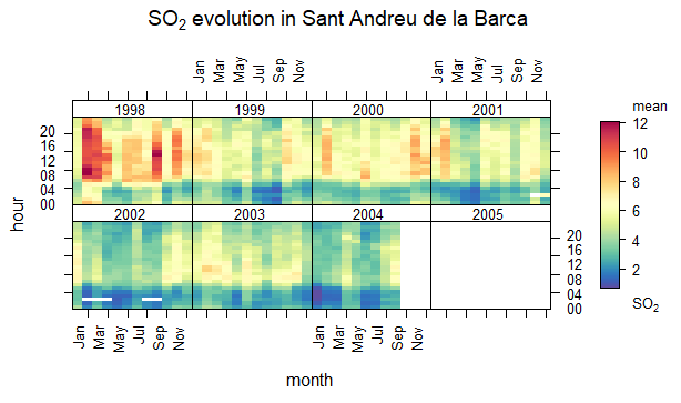  

calendarPlot

  source('C:/Users/HelenaVillaresSantia/Desktop/BACHILLERATO/1º BACHILLERATO/3er TRIMESTRE/CMC/day/datamanipulation.R', encoding = 'UTF-8')
  View(city2)
  class(city2$date)  #"POSIXct" "POSIXt"
  city2$pollutant<-as.factor(city2$pollutant)
  class(city2$pollutant)  #"factor"
  daily<-timeAverage(city2, pollutant="so2",avg.time = "day")
  View(daily)
  daily2<-replaceall(daily, c("00:00:00", "01:00:00"), c("", ""))
  daily2$date<-as.Date(daily2$date,"%Y-%m-%d", tz="Europe/Madrid")
  class(daily2)   # "tbl_df"     "tbl"        "data.frame"
  yearly<-timeAverage(daily2,avg.time = "year")
  View(yearly)    # annual average of so2 pollution in sanan
  calendarPlot(mydata, pollutant = "so2", year = 2003)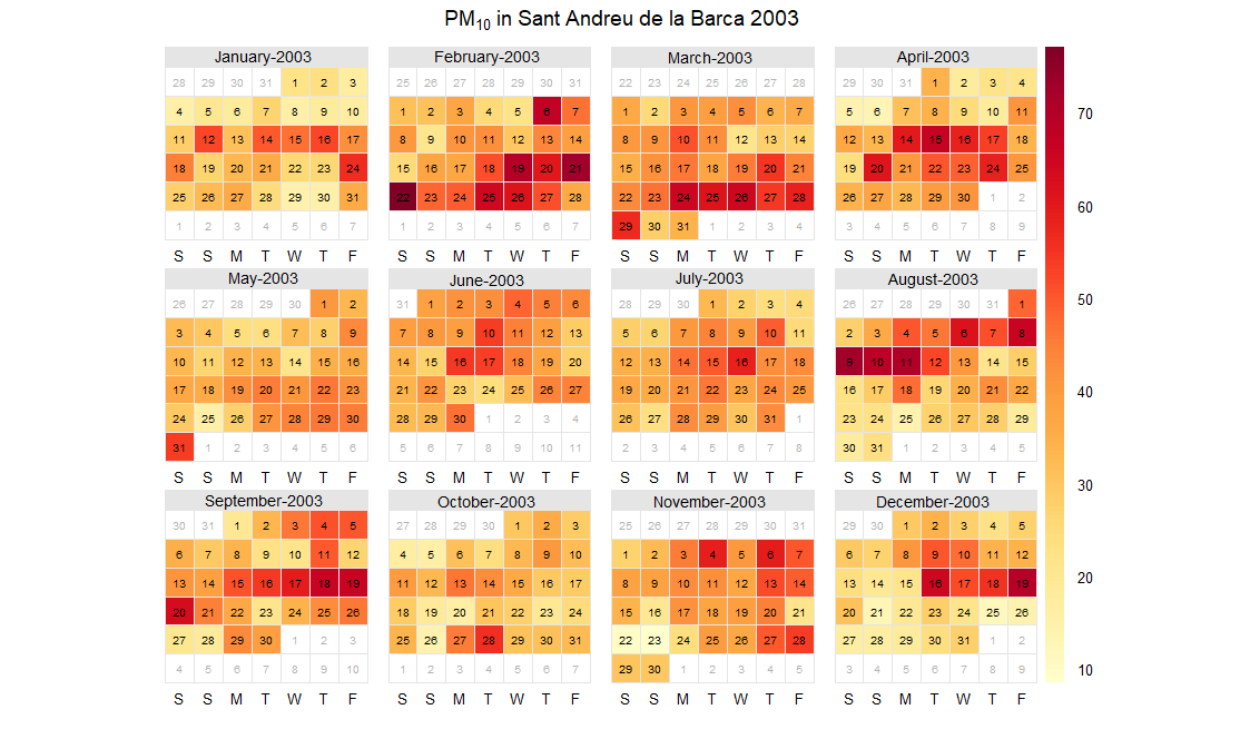  

pollutionRose

With this graph we can observe the direction of the wind and the pollution. This way we can know where large amounts of pollution come from.

  pollutionRose(cityall, pollutant="PM10")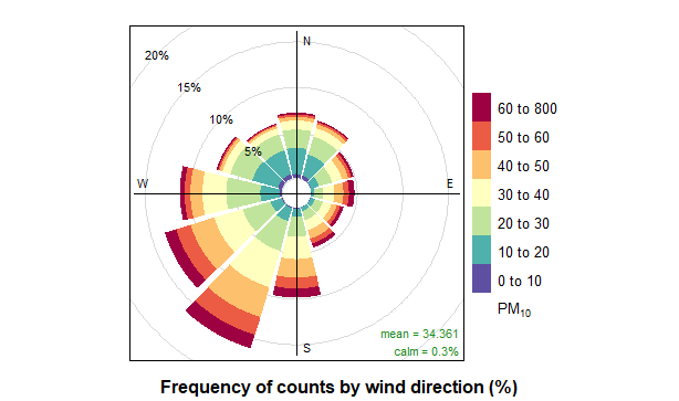  

In this case, for example, we can deduce that great quantities of PM10 come from Castellbisbal and Rubí.

PM10 is a primary pollutant, whose main emitters are traffic, construction, cement and forestry sources, among others. In Barcelona, the main sources of emissions are transport and the Port of Barcelona, which generates more than 50% of PM10 emissions.

Distribution of PM10 emissions in the city of Barcelona

timePlot

 timePlot(pivotw1,pollutant="no2")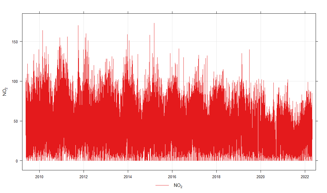 

4. Discussion

The WHO (World Health Organization), stated in 2021 the ambient outdoor air pollution limits, depending on the period and pollutant.

Europe also have its own air pollution limits.

Air pollution limits (WHO and Europe)

Pollutant (µg/m3)	Period	EU Limit	WHO Limit
PM2.5	day		15
PM2.5	year	20	5
PM10	day	50 (1)	45
PM10	year	40	15
O3	8 hours	120 (2)	60 (3)-100
NO2	hour	200 (4)	200
NO2	day		25
NO2	year	40	10
SO2	hour	350 (5)
SO2	day	125 (6)	40
CO (mg/m3)	hour		35
CO (mg/m3)	8 hours	10	10

To determine whether the pollution levels of Sant Andreu de la Barca are in the limits, the following code is executed:

 table(episodePOLLUTANT$criterion)

Whrere the pollutant is, the name of the differents pollutants must be writen (as in the following example).

From the data obtained, the percentage of hours in which the pollution levels is over the recommended limits is calculated.

5. Conclusions

From the data previously analized, it can be broadly stated that Sant Andreu de la Barca does not comply the pollution limits established from different organizations.

According to the WHO, the pollution levels of NO2 are higher than the recommended levels by more than the 66% of the hours in one year time (4) and most of the pollutants of this city are, too. PM10 goes over the recommended limits nearly the 18% of the hours. Even so, there are other pollutants, such as the ozone, which are in the limits recommended the 100% of the hours.

According to Europe, NO2 is in the recommended levels, as its criteria permits higher pollution limits (5).

6. References

1. GenCat
2. RStudio Team (2020). RStudio: Integrated Development for R. RStudio, PBC, Boston, MA
3. Conama (2014). The Local Plan for Improving Air Quality in Andreu de la Barca
4. Thw WHO (2021). Ambient (outdoor) air pollution limits
5. Europe's air quality status (2021). Pollution limits